pytorch logistic regression

import numpy as np
import torch
import torch.nn.functional as F
from torch.autograd import Variable

N = 100
D = 2

X = np.random.randn(N,D)*2

# center the first N/2 points at (-2,-2)
X[:N/2,:] = X[:N/2,:] - 2*np.ones((N/2,D))

# center the last N/2 points at (2, 2)
X[N/2:,:] = X[N/2:,:] + 2*np.ones((N/2,D))

# labels: first N/2 are 0, last N/2 are 1
T = np.array([0]*(N/2) + [1]*(N/2)).reshape(100,1)

x_data = Variable(torch.Tensor(X))
y_data = Variable(torch.Tensor(T))

class Model(torch.nn.Module):
    def __init__(self):
        super(Model, self).__init__()
        self.linear = torch.nn.Linear(2, 1) # 2 in and 1 out
        
    def forward(self, x):
        y_pred = F.sigmoid(self.linear(x))
        return y_pred
    
# Our model    
model = Model()

criterion = torch.nn.BCELoss(size_average=True)
optimizer = torch.optim.SGD(model.parameters(), lr=0.01)

# Training loop
for epoch in range(1000):
    # Forward pass: Compute predicted y by passing x to the model
    y_pred = model(x_data)
    
    # Compute and print loss
    loss = criterion(y_pred, y_data)
    print(epoch, loss.data[0])
    
    # Zero gradients, perform a backward pass, and update the weights.
    optimizer.zero_grad()
    loss.backward()
    optimizer.step()

for f in model.parameters():
    print('data is')
    print(f.data)
    print(f.grad)

w = list(model.parameters())
w0 = w[0].data.numpy()
w1 = w[1].data.numpy()

import matplotlib.pyplot as plt

print "Final gradient descend:", w
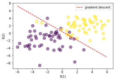
# plot the data and separating line
plt.scatter(X[:,0], X[:,1], c=T.reshape(N), s=100, alpha=0.5)
x_axis = np.linspace(-6, 6, 100)
y_axis = -(w1[0] + x_axis*w0[0][0]) / w0[0][1]
line_up, = plt.plot(x_axis, y_axis,'r--', label='gradient descent')
plt.legend(handles=[line_up])
plt.xlabel('X(1)')
plt.ylabel('X(2)')
plt.show()