Neural Convolutional layers

These are the main types of convolutional layers

Convolutional layer

Set of $n$ filters. Each filter is defined by a weight ($W$) matrix, and a bias ($b$).

Example of convolutional layer:

Output size of convolutional layer:

$W$ = input height/lenght
$K$ = filter size
$P$ = padding
$S$ = stride
$D$ = dilation

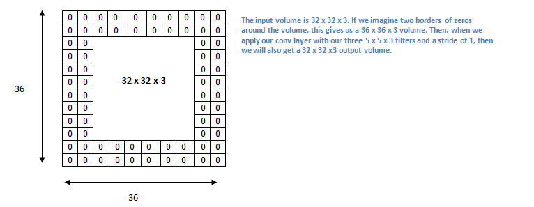
Convolutional networks with 0 padding produces a lowe dimmension output. To keep dimension equals it is convenient to put a zero padding round the border.

For example a 32x32x3 input volume we apply a 5x5x3 filter (stride = 1). Output will be (32-5)/1+1 = 28. Then output will be 28x28x3.

In order to compensate we put a padding of size 2 round the border:

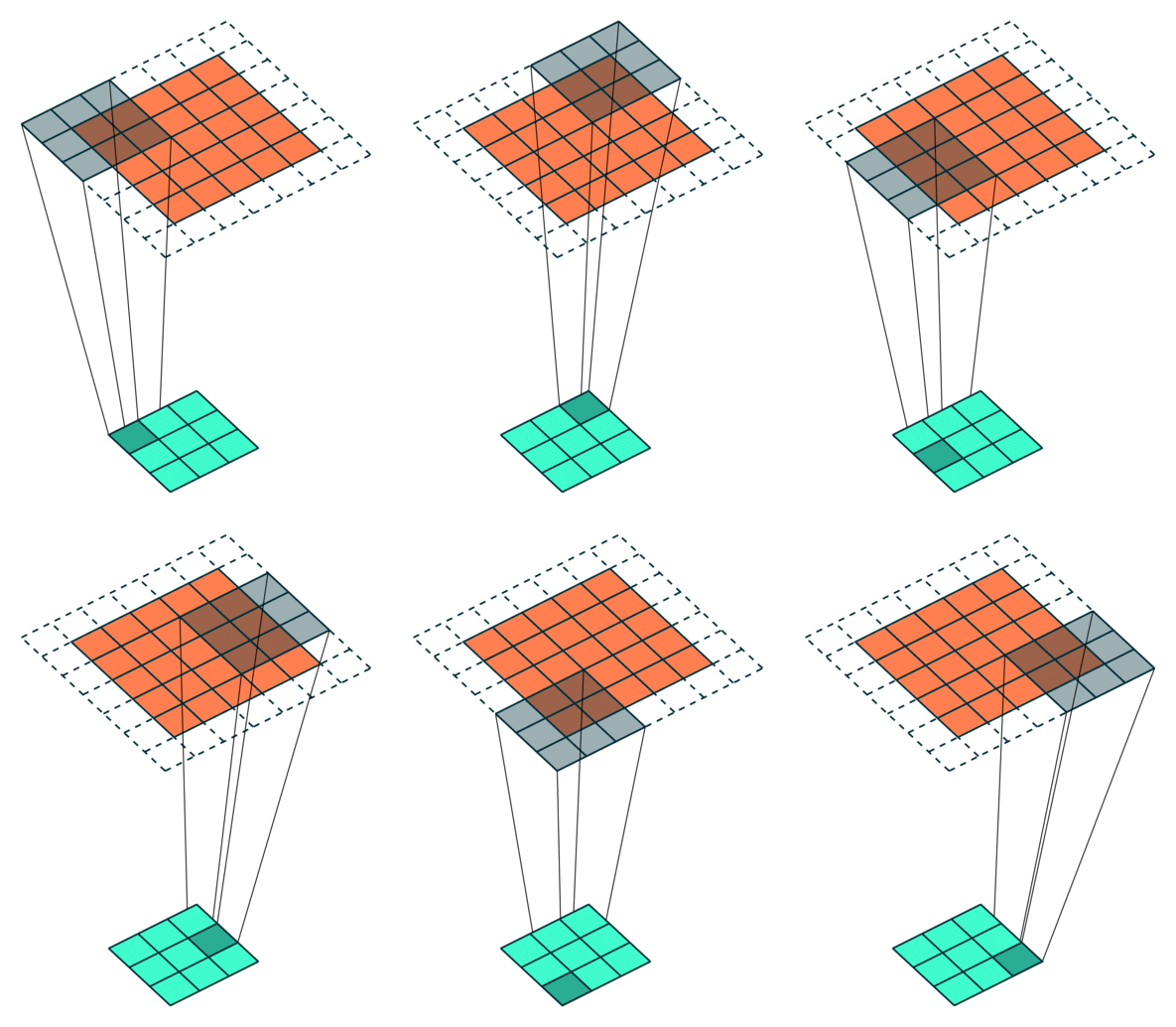
Example Stride = 2

Example Stride = 1

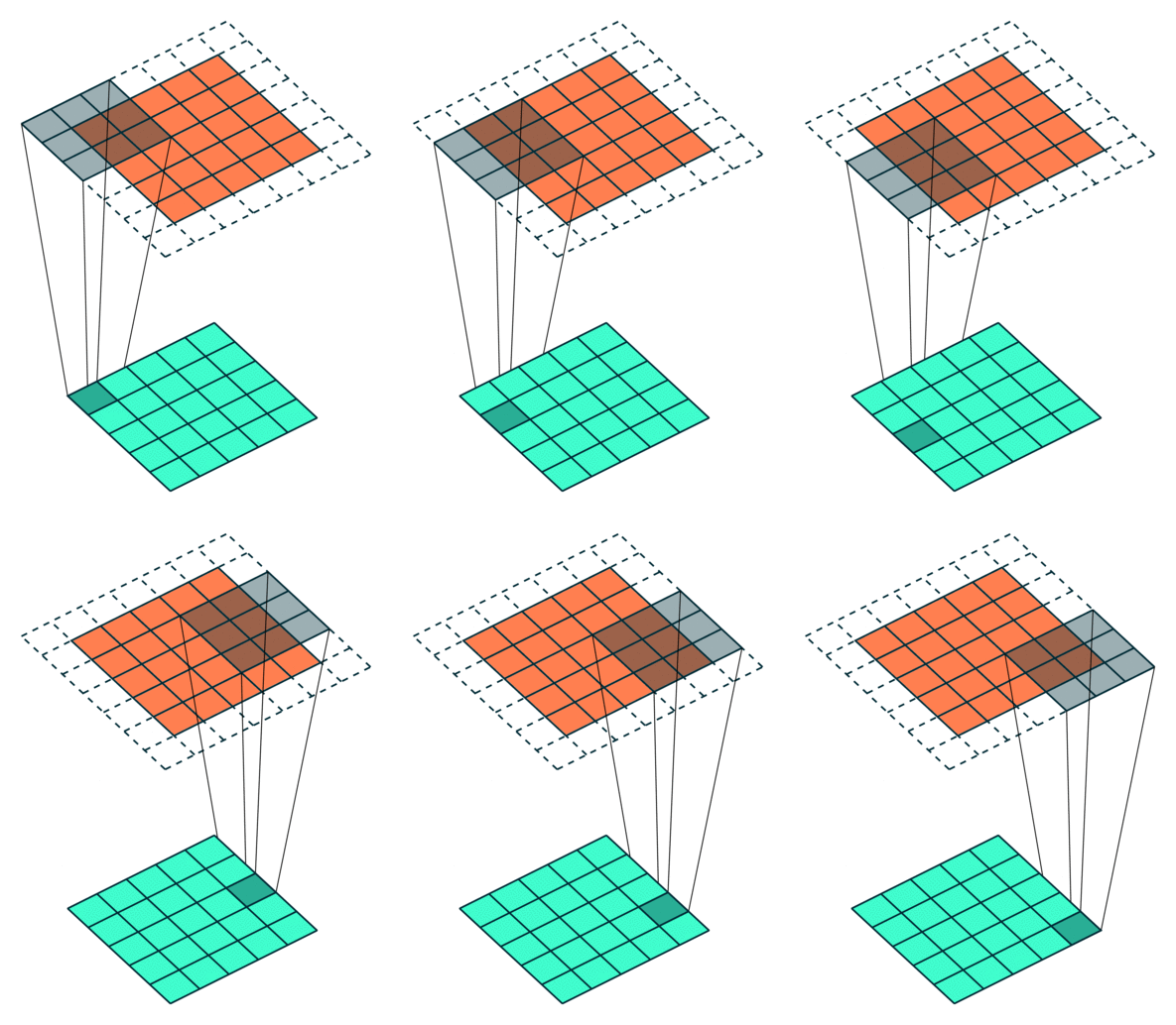
Dilation with 1, 2 3 example

Dilation animation with dilation=2

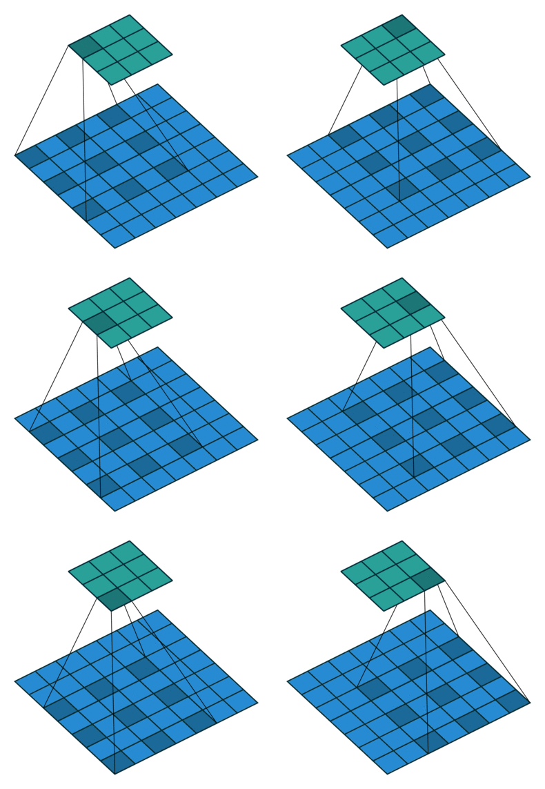
More examples of convolution arithmetic:

arithmetic examples

Convolution layers incorporate following key features:

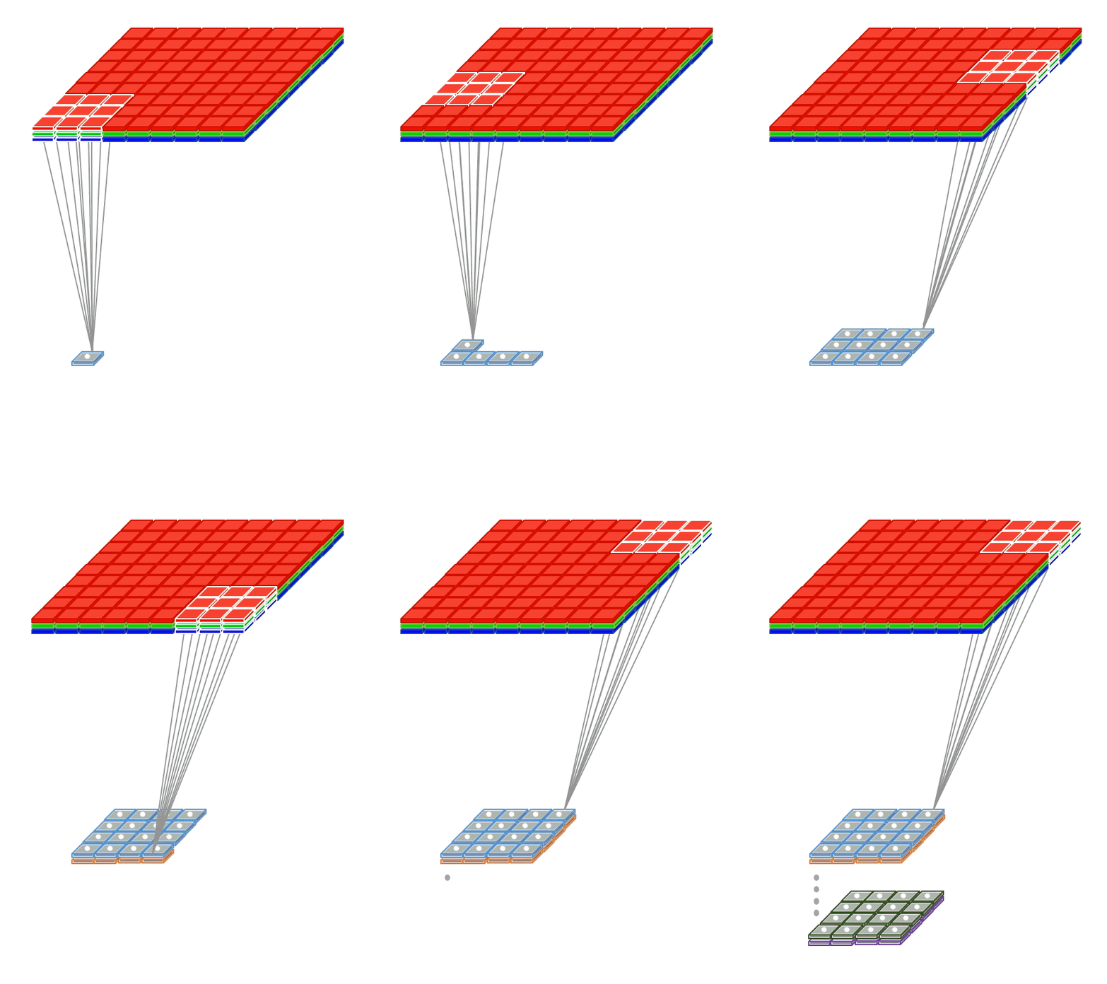
• Instead of being fully-connected to all pairs of input and output nodes , each convolution node is locally-connected to a subset of input nodes localized to a smaller input region, also referred to as receptive field (RF). The figure above illustrates a small 3 x 3 regions in the image as the RF region. In the case of an RGB, image there would be three such 3 x 3 regions, one each of the 3 color channels.

• Instead of having a single set of weights (as in a Dense layer), convolutional layers have multiple sets (shown in figure with multiple colors), called filters. Each filter detects features within each possible RF in the input image. The output of the convolution is a set of n sub-layers (shown in the animation below) where n is the number of filters (refer to the above figure).

• Within a sublayer, instead of each node having its own set of weights, a single set of shared weights are used by all nodes in that sublayer. This reduces the number of parameters to be learnt and thus overfitting. This also opens the door for several aspects of deep learning which has enabled very practical solutions to be built: – Handling larger images (say 512 x 512) - Trying larger filter sizes (corresponding to a larger RF) say 11 x 11 - Learning more filters (say 128) - Explore deeper architectures (100+ layers) - Achieve translation invariance (the ability to recognize a feature independent of where they appear in the image).

Pooling layer

Often a times, one needs to control the number of parameters especially when having deep networks. For every layer of the convolution layer output (each layer, corresponds to the output of a filter), one can have a pooling layer. Pooling layers are typically introduced to:

• Reduce the dimensionality of the previous layer (speeding up the network),
• Makes the model more tolerant to changes in object location in the image. For example, even when a digit is shifted to one side of the image instead of being in the middle, the classifer would perform the classification task well.

The calculation on a pooling node is much simpler than a normal feedforward node. It has no weight, bias, or activation function. It uses a simple aggregation function (like max or average) to compute its output. The most commonly used function is “max” - a max pooling node simply outputs the maximum of the input values corresponding to the filter position of the input. The figure below shows the input values in a 4 x 4 region. The max pooling window size is 2 x 2 and starts from the top left corner. The maximum value within the window becomes the output of the region. Every time the model is shifted by the amount specified by the stride parameter (as shown in the figure below) and the maximum pooling operation is repeated.

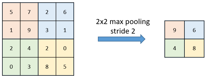
Example for max and average pooling:

Dropout Layer

Dropout layers consists in randomly setting a fraction $rate$ of inputs to $0$ at each update during training time, which helps prevent overfitting. It forces the network to be redundant.

sources:
microsoft CNTK
A Beginner’s Guide To Understanding Convolutional Neural Networks Part 2