sgd momentum comparison
2 Jan 2018
This post is to show a quick python example comparison between standard and momentum stochastic gradient descent.
Gradient descent formula:
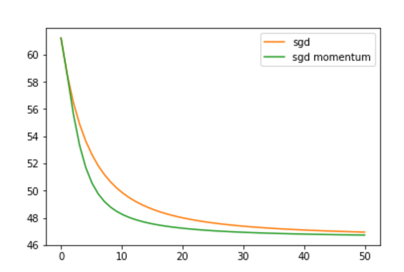
Python example that shows that momentum version gets faster to converge:
import numpy as np
import matplotlib.pyplot as plt
import pandas as pd

def sigmoid(z):
    return 1/(1 + np.exp(-z))

# View images

# calculate the cross-entropy error
def cross_entropy(T, Y):
    E = 0
    for i in xrange(len(T)):
        if T[i] == 1:
            E -= np.log(Y[i])
        else:
            E -= np.log(1 - Y[i])
    return E

N = 200
D = 2
iter = 50

X = np.random.randn(N,D)*2

# center the first 50 points at (-2,-2)
X[:N/2,:] = X[:N/2,:] - 2*np.ones((N/2,D))

# center the last 50 points at (2, 2)
X[N/2:,:] = X[N/2:,:] + 2*np.ones((N/2,D))

# labels: first N/2 are 0, last N/2 are 1
T = np.array([0]*(N/2) + [1]*(N/2))

# add a column of ones
# ones = np.array([[1]*N]).T # old
ones = np.ones((N, 1))
Xb = np.concatenate((ones, X), axis=1)

# randomly initialize the weights
w_base = np.random.randn(D + 1)


w = w_base.copy()

print "w:", w

# calculate the model output
z = Xb.dot(w)


Y = sigmoid(z)
# let's do gradient descent 100 times
learning_rate = 0.001
costs = []

for i in xrange(iter):
    costs.append(cross_entropy(T, Y))

    # gradient descent weight udpate
    w += learning_rate * Xb.T.dot(T - Y)

    # recalculate Y
    Y = sigmoid(Xb.dot(w))


w2 = w_base.copy()

print "w2:", w2


# calculate the model output
z = Xb.dot(w2)


Y = sigmoid(z)
# let's do gradient descent 100 times
learning_rate = 0.001
gamma = 0.4
costs2 = []
v = np.zeros(D + 1)
for i in xrange(iter):
    costs2.append(cross_entropy(T, Y))

    v = learning_rate*Xb.T.dot(T - Y) + gamma*v

    # gradient descent weight udpate
    w2 += v

    # recalculate Y
    Y = sigmoid(Xb.dot(w2))


print "Final gradient descend sgd         :", w
print "Final gradient descend sgd momentum:", w2
# plot the data and separating line
plt.scatter(X[:,0], X[:,1], c=T, s=100, alpha=0.5)
x_axis = np.linspace(-6, 6, 100)
y_axis = -(w[0] + x_axis*w[1]) / w[2]
line_up, = plt.plot(x_axis, y_axis,'r--', label='sgd')
y_axis = -(w2[0] + x_axis*w2[1]) / w2[2]
line_down, = plt.plot(x_axis, y_axis,'g--', label='sgd with momentum')
plt.legend(handles=[line_up, line_down])
plt.xlabel('X(1)')
plt.ylabel('X(2)')
plt.title('regression')
plt.show()

th = np.linspace(0, iter, iter)
plt.plot(th, costs, 'C1', label='sgd')
plt.plot(th, costs2, 'C2', label='sgd momentum')
plt.legend()
plt.set_title('style: {!r}'.format('default'), color='C0')
plt.title('cross entropy')
plt.show()
This is a comparison of other algorithms extracted from here