Gradiend descent

Demonstration of normal (Batch) gradient descend formulas

$y$ is the training input (always 0 or 1)
$m$ is the size of de dataset input x
$w$ are the parameters of logistic regression

First assumption is that can aproximate the likehood with the sigmoid function:

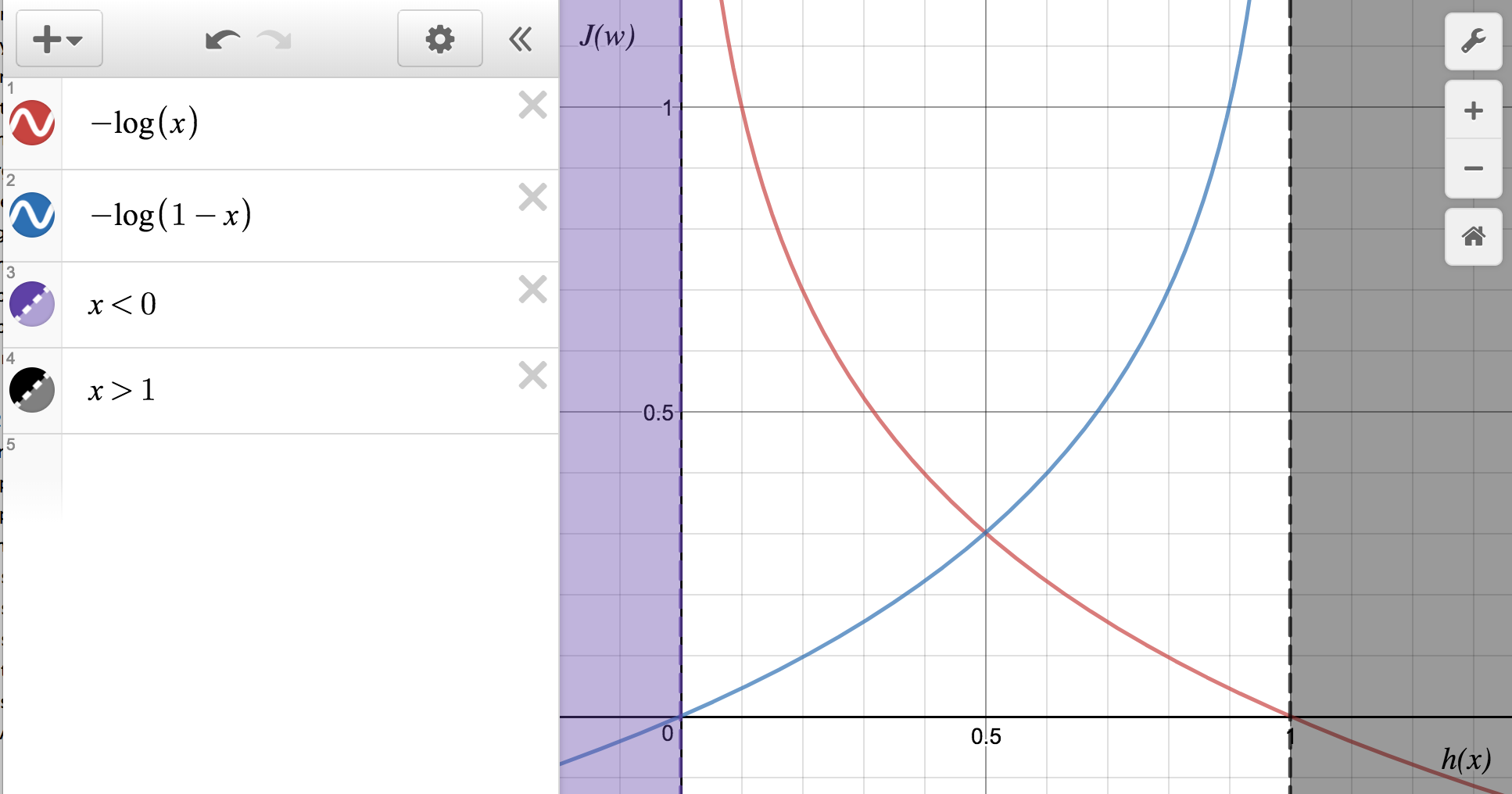
$\text{Likelihood} = h_w(x_i) = sigmoid(x_i^\intercal w)={1 \over 1-e^{-x_i^\intercal w}} \text{ }\text{ }\text{ }\forall i \in 1..m$

Cost funcion (is the likelihood negated) is the error on every iteration (cross entropy error) and depends on likelihood.

$J_i(w) = \mathrm{Cost}(h_w(x_i),y_i) \text{ }\text{ }\text{ }\forall i \in 1..m$ $J(w) = \dfrac{1}{m} \sum_{i=1}^m \mathrm{Cost}(h_w(x_i),y_i)$ $\mathrm{Cost}(h_w(x),y) = \begin{cases} -\log(h_w(x)) & \text{if $y = 1$,} \\ -\log(1-h_w(x)) & \text{if $y = 0.$} \end{cases}$

graphic of cost

$\bbox[5px,border:2px solid black] {\begin{align*}& \mathrm{Cost}(h_w(x),y) = 0 \text{ if } h_w(x) = y \newline & \mathrm{Cost}(h_w(x),y) \rightarrow \infty \text{ if } y = 0 \; \mathrm{and} \; h_w(x) \rightarrow 1 \newline & \mathrm{Cost}(h_w(x),y) \rightarrow \infty \text{ if } y = 1 \; \mathrm{and} \; h_w(x) \rightarrow 0 \newline \end{align*}}$

This formula is derived from calculation of likelihood of the $m$ inputs as:

$P(Y=1|X)=\prod_{i=1}^N \prod_{k=1}^2 h_k(x^{(i)})^{y_k^{(i)}}$

Note: we assume that the output has an output binary class k = 2, that have redundant and opposed probabilities.

$ln(P(Y=1|X))=\sum_{i=1}^N \sum_{k=1}^2 y_k^{(i)}ln(h_k(x^{(i)}))$ $ln(P(Y=1|X))=\sum_{i=1}^N (y_1^{(i)}ln(h_1(x^{(i)}))+(1-y_1^{(i)})ln(1-h_1(x^{(i)})))$

Retuning to the cost ($J(w)$):

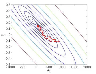
$J(w) =-\frac{1}{m} \cdot \sum_{i=1}^m\Bigl( y_i log(h_i)+(1-y_i)log(1-h_i)\Bigl)$ $J(w) = \frac{1}{m} \cdot \left(-y_{M\times 1}^\intercal \log(h_w(x)_{M\times 1})-(1-y_{M\times 1})^\intercal \log(1-h_w(x)_{M\times 1})\right)$

There is a global minimum thar can be achieved using gradient descent.

$\begin{align*}& Repeat \; \lbrace \newline & \; w_j := w_j - \alpha \dfrac{\partial}{\partial w_j}J(w) \newline & \rbrace\end{align*}$ $f(x) = log_a(g(x)) \rightarrow f'(x) = \dfrac {g'(x)}{g(x)}log_ae$ $\dfrac{\partial}{\partial w_j}J(w) =\dfrac{\partial}{\partial w_j} \Biggl(\dfrac{-1}{m} \sum_{i=1}^m \mathrm{Cost}(h_w(x_i),y_i)\Biggl)$ $=\dfrac{-log_ae}{m}\sum_{i=1}^m {y_i \dfrac{1}{\require{cancel}\cancel {h_w(x_i)}}\cancel {h_w(x_i)}(1-h_w(x_i))x_j+ (1-y_i) \dfrac{1}{1-h_w(x_i)}h_w(x_i)(h_w(x_i)-1)x_j}$ $=\dfrac{-log_ae}{m}\sum_{i=1}^m {y_i(1-h_w(x_i))x_j- (1-y_i) \dfrac{1}{\cancel{1-h_w(x_i)}}h_w(x_i)(\cancel{1-h_w(x_i)})x_j}$ $=\dfrac{-log_ae}{m}\sum_{i=1}^m {y_i(1-h_w(x_i))x_j- (1-y_i)h_w(x_i)x_j}$ $=\dfrac{log_ae}{m}\sum_{i=1}^m {(h_w(x_i)-y_i)x_j}$ $\begin{align*} & Repeat \; \lbrace \newline & \; w_j := w_j - \frac{\alpha}{m} \sum_{i=1}^m (h_w(x^{(i)}) - y^{(i)}) x_j^{(i)} \newline & \rbrace \end{align*}$ $w := w_{J\times 1} - \frac{\alpha}{m} X_{M\times J}^\intercal (h_{M\times 1} - y_{M\times 1})$ $w := w_{J\times 1} + \gamma X_{M\times J}^\intercal (y_{M\times 1} - h_{M\times 1})$

There are several types of gradient descent implementation:

Batch gradient descent: iteration (new coefs) is done as the sum of all training examples
Stochastic gradient descent: iteration on each example, converges faster than batch gradient descent in case of large training dataset.
Mini-batch gradient descent: iteration on a group of $b$ examples, in some cases can converge faster than batch or stochastic.
Stochastic gradient descent with momentum: each gradient has a momentum added from the previous gradient:

$\begin{align} \begin{split} v_t &= \gamma v_{t-1} + \eta \nabla_\theta J( \theta) \\ \theta &= \theta - v_t \end{split} \end{align}$

Important implementation concepts:

Debug results to adjust the learning rate
Possibly set dinamic learning rate as: $\alpha = \dfrac{const_1}{interationNumber + const_2}$ so learning rate decreases as it aproaches to the minimum.

dynamic alpha

An special case of stochastic gracient descent is the Online learning. Learning is done continuously from a source flow that generates training examples. Each example is used for train and ignored (not stored).

source: coursera machine learning course

Glosary

MLE: Maximum Likelihood Estimation
sigmoid: function to map $[-\infty,\infty]$ to $[0,1]$
Epoch: Epoch means one iteration of Stochastic Gradient Descent