Logistic Regression (Logit)

Binary Logistic Regression is aplied to classification problems, in which there are a list of numerical (Real, integers) features that are related to the classification of one boolean output Y[0,1].

Logistic regresion is fine for linealy separable problems, since is a linear clasifier:

2D: bounday is a line (as the example in this post)
3D: bounday is a plane
4D-nD: bounday is a hyperplane
all of them are linear, not curved.

Another way to see a logistic regression is the neuron (sigmoid), with $X_n+1$ inputs and a unique binary output.

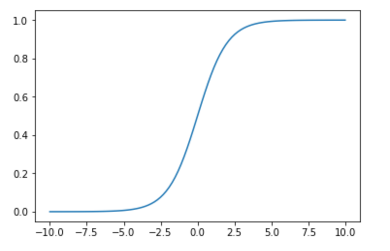
Logit function is an useful function that maps an unlimited input to a binary value Y. The logit function is the natural log of the odds that Y equals to 0 or 1. This useful function (called sigmoid) compress the $[-\infty,\infty]$ variance of $\beta+\beta_1x_1+\beta_2x_2+…+\beta_kx_k$ to a $[0,1]$ field that is the probability P that output value equals to 1. There is a much better explanation here.

$\text{logit}(P) = ln\left(odds\right) = ln\left({P \over 1-P}\right)=\beta+\beta_1x_1+\beta_2x_2+...+\beta_kx_k$

Clearing P variable show the sigmoid formula:

$P(Y=1|X^{(i)}) = {1 \over 1+ e^{-(\beta+\beta_1x^{(i)}_1+\beta_2x^{(i)}_2+...+\beta_kx^{(i)}_k)}}$

sigmoid

In this article I’m interested in the result from the hand made regression with the above formula versus the common python libraries.

import numpy as np
import matplotlib.pyplot as plt
import pandas as pd

import statsmodels.api as sm
from scipy import stats
stats.chisqprob = lambda chisq, df: stats.chi2.sf(chisq, df)

from sklearn.linear_model import LogisticRegression
from sklearn.cross_validation import train_test_split

def sigmoid(z):
    return 1/(1 + np.exp(-z))

# View images

# calculate the cross-entropy error
def cross_entropy(T, Y):
    E = 0
    for i in xrange(len(T)):
        if T[i] == 1:
            E -= np.log(Y[i])
        else:
            E -= np.log(1 - Y[i])
    return E

N = 100
D = 2

X = np.random.randn(N,D)*2

# center the first 50 points at (-2,-2)
X[:N/2,:] = X[:N/2,:] - 2*np.ones((N/2,D))

# center the last 50 points at (2, 2)
X[N/2:,:] = X[N/2:,:] + 2*np.ones((N/2,D))

# labels: first N/2 are 0, last N/2 are 1
T = np.array([0]*(N/2) + [1]*(N/2))

# add a column of ones
# ones = np.array([[1]*N]).T # old
ones = np.ones((N, 1))
Xb = np.concatenate((ones, X), axis=1)

# randomly initialize the weights
w = np.random.randn(D + 1)

# calculate the model output
z = Xb.dot(w)


Y = sigmoid(z)
# let's do gradient descent 100 times
learning_rate = 0.1
for i in xrange(100):
    if i % 10 == 0:
        print cross_entropy(T, Y)

    # gradient descent weight udpate
    w += learning_rate * Xb.T.dot(T - Y)

    # recalculate Y
    Y = sigmoid(Xb.dot(w))



y2 = pd.Series(T.tolist())
X2 = pd.concat([pd.Series(Xb[:,1].tolist()), pd.Series(Xb[:,2].tolist())], axis=1)

X2 = sm.add_constant(X2)
logit_model=sm.Logit(y2,X2)
result=logit_model.fit()
print(result.summary())
print(result.conf_int())

w2 = result.params.values

X_train, X_test, y_train, y_test = train_test_split(X, T, test_size=0.3, random_state=0)
logreg = LogisticRegression()
logreg.set_params(solver='sag').fit(X_train, y_train)

w3 = np.append(logreg.intercept_,logreg.coef_)

print "Final gradient descend:", w
print "Final statsmodels:", w2
print "Final sklearn:", w3
# plot the data and separating line
plt.scatter(X[:,0], X[:,1], c=T, s=100, alpha=0.5)
x_axis = np.linspace(-6, 6, 100)
y_axis = -(w[0] + x_axis*w[1]) / w[2]
line_up, = plt.plot(x_axis, y_axis,'r--', label='gradient descent')
y_axis = -(w2[0] + x_axis*w2[1]) / w2[2]
line_down, = plt.plot(x_axis, y_axis,'g--', label='statsmodels')
y_axis = -(w3[0] + x_axis*w3[1]) / w3[2]
line_down2, = plt.plot(x_axis, y_axis,'b--', label='sklearn')
plt.legend(handles=[line_up, line_down, line_down2])
plt.xlabel('X(1)')
plt.ylabel('X(2)')
plt.show()

Note: source

results graphic

results summary

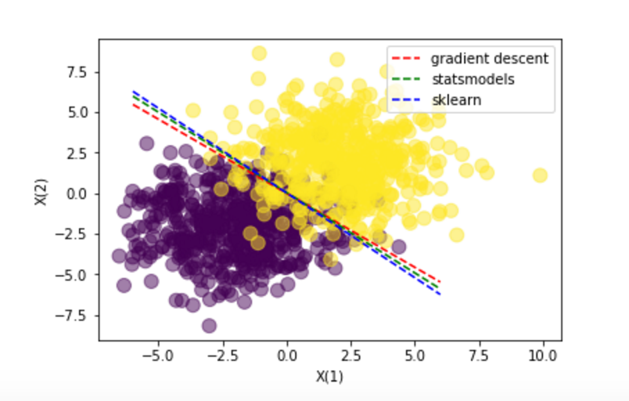
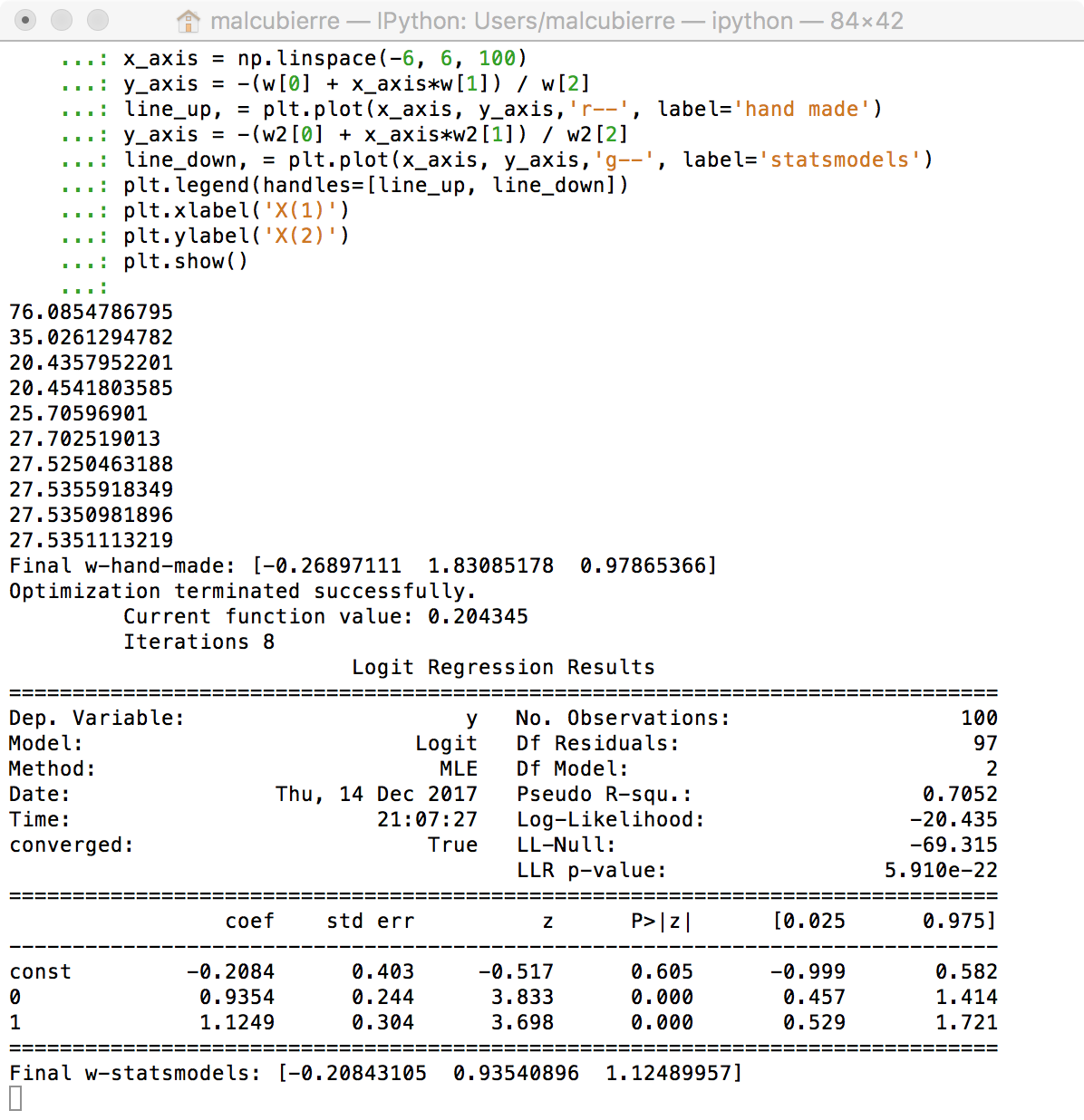
Conclusions: All methods guide us to the same resuls. The manual way through the Gradient descent, the Statsmodels through the Newton-Raphson algorithm (that has some probles with Perfect separation examples) and the Sklear with a similar gradient descent.

Here a good explanation for z and p-values. Good values for z are < 0.05.